7. Mask creation & Post processing

After performing a 3D auto-refinement, the map needs to be sharpened. Also, the gold-standard FSC curves inside the auto-refine procedures only use unmasked maps (unless you’ve used the option Use solvent-flattened FSCs). This means that the actual resolution is under-estimated during the actual refinement, because noise in the solvent region will lower the FSC curve. Relion’s procedure for B-factor sharpening and calculating masked FSC curves (Chen et al, 2013) is called post-processing. First however, we’ll need to make a mask to define where the protein ends and the solvent region starts. This is done using the Mask Creation job-type.

7.1. Making a mask

In the Mask Creation category select RELION mask create job and set the following parameters:

Input 3D map:: Refine3D/job019/run_class001.mrc
NOTE: Use the full map from your Refine3D job.

Lowpass filter map (A):: 15
NOTE: A 15 Å low-pass filter seems to be a good choice for smooth solvent masks for many proteins.

Pixel size (A):: -1
NOTE: This value will be taken automatically from the header of the input map.

Initial binarisation threshold:: 0.01
NOTE: This should be a threshold at which rendering of the low-pass filtered map in e.g. chimera shows no noisy spots outside the protein area. Move the threshold up and down to find a suitable spot. Often good values for the initial threshold are around 0.002-0.02.

Extend binary map this many pixels:: 3
NOTE: The threshold above is used to generate a black-and-white mask. The white volume in this map will be grown this many pixels in all directions. Use this to make your initial binary mask less tight.

Add a soft-edge of this many pixels:: 8
NOTE: This will put a cosine-shaped soft edge on your masks. This is important, as the correction procedure that measures the effect of the mask on the FSC curve may be quite sensitive to too sharp masks. As the mask generation is relatively quick, we often play with the mask parameters to get the best resolution estimate.

HEADER: Running options

Number of threads:: 10
NOTE: This will speed up the calculation.

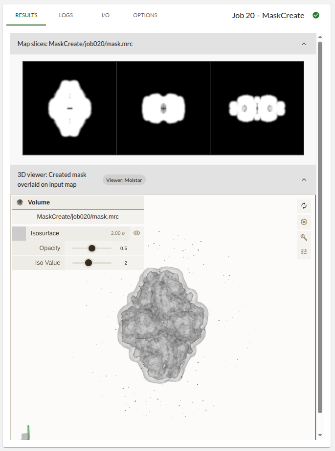
This should take <2 mins to run. It took 10 seconds on the tested system. When the job is complete click on the RESULTS tab. You can see the mask in the first section, and the mask overlaid on the input map on the 3D viewer. Make sure the mask encapsulates the entire structure but does not leave a lot of solvent inside the mask. Also ensure the mask does not have the high-resolution features present in the input map. You repeat with different settings until you are happy.

7.2. Post-processing

In Map Postprocessing select a new RELION Post-processing job and set the following:

One of the 2 unfiltered half-maps:: Refine3D/job019/run_half1_class001_unfil.mrc

Solvent mask:: MaskCreate/job020/mask.mrc

Calibrated pixel size (A):: 1.244
NOTE: Sometimes you find out when you start building a model that what you thought was the correct pixel size, in fact was off by several percent. Inside Relion, everything up until this point was still consistent. so you do not need to re-refine your map and/or re-classify your data. All you need to do is provide the correct pixel size here for your correct map and final resolution estimation.

Estimate B-factor automatically:: Yes
NOTE: This procedure is based on the classic 2003 Rosenthal and Henderson paper, and will need the final resolution to extend significantly beyond 10 Å. If your map does not reach that resolution, you may want to use your own ad-hoc B-factor instead.

Lowest resolution for auto-B fit (A):: 10
NOTE: This is usually not changed.

Use your own B-factor?:: No

MTF of the detector (STAR file):: mtf_k2_200kV.star
NOTE: This file came from the microscope.

Original detector pixel size:: 0.885
NOTE: This is the original pixel size (in Angstroms) in the raw (non-super-resolution!) micrographs.

Skip FSC-weighting?:: No
NOTE: This option is sometimes useful to analyse regions of the map in which the resolution extends beyond the overall resolution of the map. This is not the case now.

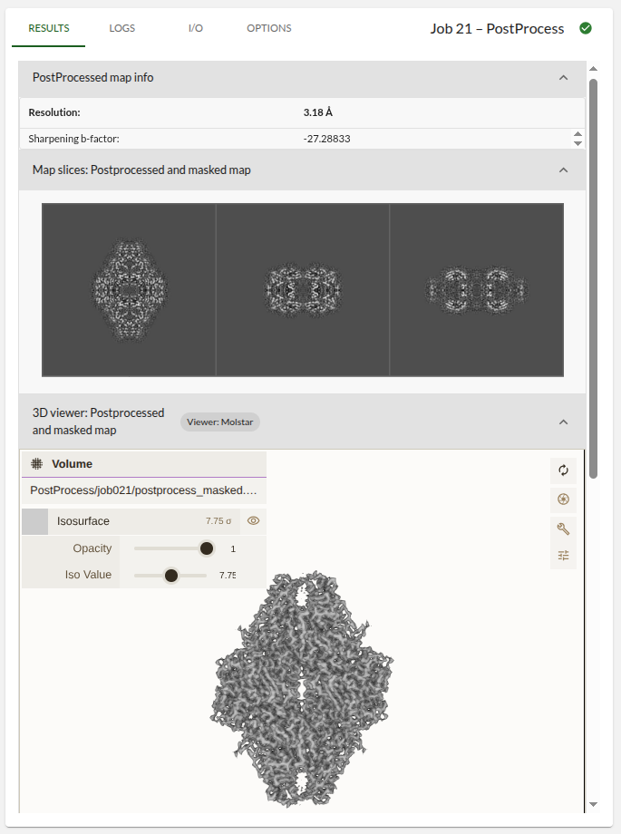
Press RUN, the job should take less than 10 seconds to run. Now look at the RESULTS tab. You’ll see the improvement in resolution estimate from masking out the noisy solvent regions in the two half maps, the resolution should be around 3.18A.

If you’re having trouble viewing the model in Mol*, check out these solutions.

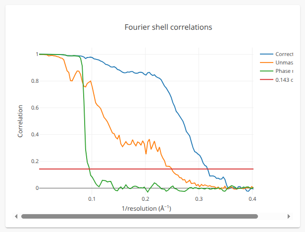
You can also see this improvement in resolution. Take a look at the FSC plot. The resolution estimate is based on the phase-randomization procedure as published previously (Chen et al, 2013). Make sure that the FSC of the phase-randomised maps (the green curve) is more-or-less zero at the estimated resolution of the postprocessed map. If it is not, then your mask is too sharp or has too many details. In that case use a stronger low-pass filter (i.e. lower resolution, for example from 50Å to 70Å ) and/or a wider and softer mask in the Mask creation step above and repeat the postprocessing.