5. Unsupervised 3D classification

All data sets are heterogeneous! The question is how much you are willing to tolerate. Relion’s 3D multi-reference refinement procedure provides a powerful unsupervised 3D classification approach.

5.1. Class 3D

In the 3D Classification section of New Job select the RELION 3D classification (single particle). Setup with the following parameters:

Input images STAR file:: Select/job013/particles.star

Reference map:: InitialModel/job014/initial_model.mrc
NOTE: Use the initial model job you ran previously.

Ref. map is on absolute greyscale:: Yes
NOTE: Given that this map was reconstructed from this data set, it is already on the correct greyscale. Any map that is not reconstructed from the same data in Relion should probably be considered as not being on the correct greyscale.

Reference mask (optional):: <leave blank>
NOTE: This is the place where we for example provided large/small-subunit masks for our focussed ribosome refinements. If left empty, a spherical mask with the particle diameter given below will be used. This introduces the least bias into the classification.

Initial low-pass filter (A):: 50
NOTE: One should NOT use high-resolution starting models as they may introduce bias into the refinement process. As also explained in (Scheres 2010), one should filter the initial map as much as one can. For ribosome we often use 70 Å, for smaller particles we typically use values of 40-60 Å.

Symmetry:: C1
NOTE: Although we know that this sample has D2 symmetry, it is often a good idea to perform an initial classification without any symmetry, so bad particles, which are not symmetric, can get separated from proper ones, and the symmetry can be verified in the reconstructed maps.

Do CTF correction?:: Yes

Ignore CTFs until first peak?:: No
NOTE: Only use this option if you also did so in the 2D classification job that you used to create the references.

Number of classes:: 4
NOTE: Using more classes will divide the data set into more subsets, potentially describing more variability. The computational costs scales linearly with the number of classes, both in terms of CPU time and required computer memory.

Regularisation parameter T:: 4
NOTE: For the exact definition of T, please refer to Scheres, 2012a (A Bayesian view...). For cryoEM 2D classification we typically use values of T=1-2, and for 3D classification values of 2-4. For negative stain sometimes slightly lower values are better. In general, if your class averages appear noisy, then lower T; if your class averages remain too low resolution, then increase T. The main thing is to be aware of overfitting high-resolution noise.

Number of iterations:: 25
NOTE: We typically do not change this.

Mask diameter (A):: 200
NOTE: Just use the same value as we did before in the 2D classification job-type.

Mask individual particles with zeros?:: Yes

Limit resolution E-step to (A):: -1
NOTE: If a positive value is given, then no frequencies beyond this value will be included in the alignment. This can also be useful to prevent overfitting. Here we don’t really need it, but it could have been set to 10-15Å anyway.

Angular sampling interval:: 7.5 degrees

Offset search range (pix):: 5

Offset search step (pix):: 1

Perform local angular searches?:: No

Allow coarser sampling?:: No
NOTE: The above are all set to the default values which rarely change except for large and highly symmetric particles, like icosahedral viruses, where 3.7 degrees angular sampling is typically used.

HEADER: Compute options

Use parallel disc I/O?:: Yes

Number of pooled particles:: 30

Skip padding?:: No

Skip gridding?:: Yes

Pre-read all particles into RAM?:: No
NOTE: Again, this is only possible if the data set is small and/or you have a large amount of memory.

Copy particles to scratch directory:: <leave blank>
NOTE: N.B. If your computer does not have enough RAM, you may need to fill this option

Combine iterations through disc?:: Yes

Use GPU acceleration?:: Yes

Which GPUs to use:: <leave blank>

HEADER: Running options

Number of threads:: 2

Number of MPI procs:: 5
NOTE: As before, you should set this to one plus the number of GPUs you want to use.

Click RUN to start the job. Using the settings above, this job took ~7 minutes on the STFC VMs.

Once completed in the RESULTS panel you can view the particle class distribution and the 3D maps for each 3D class. From the distribution plots see how many particles have been selected for each class and if the selection has converged. The 3D map(s) of the major class(es) allow you to check they have the expected shape.

5.2. Selecting good particles for further processing:

When you are ready to choose your class(es) launch 3D class auto selection via the NEW JOB menu from Automated Class Selection category.

Input 3D classification particles file:: Class3D/job015/run_it25_data.star

Then press RUN. The job should take less than 10 seconds to execute. Once the job has finished, the RESULTS tab will once again show a montage of selected 3d averages.

This job selects the particles from the highest resolution 3D class. In most cases this will give the best result. After the job has completed, compare the selected class to the classes in the previous 3D classification job. Did the job select the best 3D class?

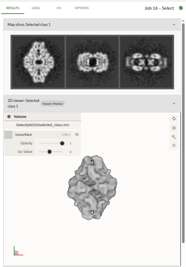
If you’re having trouble viewing the model in Mol*, check out these solutions.