7. Optional: Checking disordered loop regions using LAFTER map

Another interesting area to work on is the loop in the region spanning ~Ala726 to ~Ala737. This is hard to model as the density is weaker here, most likely caused by local disorder in the flexible loop. Here it is useful to use the denoised LAFTER map.

7.1. LAFTER map preparation

It’s often useful to make various additional maps to help with visualisation and interpretation. These can range from quite simple and “safe” operations such as global B-factor sharpening or blurring, through to more “dangerous” map enhancements that can claim to increase the map resolution or improve the clarity of map features, but with the risk of hallucinating realistic-looking features that are not actually supported by the experimental data.

Here we will run one tool called LAFTER, which is quite a safe option. It locally denoises maps by identifying features in each resolution shell that are shared between the two half maps, so you can reasonably interpret the output as a consensus map – if a feature is present in the LAFTER map it means that it is present in both half maps and so is unlikely to be purely noise. This can be a useful complement to sharpened or enhanced maps, to check that you are not optimistically interpreting noise peaks as real molecular density.

If you ran LAFTER earlier in the tutorial, no need to run it again. You can use the output map from that job in the next section! If not, find the LAFTER job (in the Map Postprocessing section) and enter the following options:

Input map 1 (half map 1):: Refine3D/job029/run_half1_class001_unfil.mrc
Input map 2 (half map 2):: Refine3D/job029/run_half2_class001_unfil.mrc
Input mask:: MaskCreate/job020/mask.mrc

Run the job. Have a look at the output map now if you like, but it will be most useful to load it into Moorhen or Coot later when looking at fitted and refined models as an aid to interpretation.

Servalcat also produces a “normalised expected map” from each refinement job. This is a map that is globally sharpened based on the variance between the two half maps. In well-resolved regions it often looks very similar to the LAFTER map, but in regions with low local resolution they can be quite different. In those areas, LAFTER is usually a good guide to the reliable low-resolution features, while the post-processed and Servalcat maps can show higher-resolution features that should be interpreted with caution.

7.2. LAFTER map in Moorhen

Open the maps and model again: from the I/O tab of the previous Moorhen job, select the input refined_maps.mtz file and the output refined_moorhen.pdb, then click the Moorhen (beta) button. (We are not using the Edit in Moorhen button on the Results tab because Moorhen doesn’t currently reload difference maps properly when opening a previous session.) Use the Doppio Files menu to select the Density Map from the LAFTER job. Go to the loop region (spanning ~Ala726 to ~Ala737) and compare the normalized Servcalcat map with the denoised LAFTER map. Test different contour levels and you should find the LAFTER map shows more contiguous density in this region, with fewer noise peaks. N.B. it is useful to change the colour of the LAFTER map (shown below in pink). You can also open up the initial postprocessed map from RELION for comparison, which appears substantially more noisy in this region.

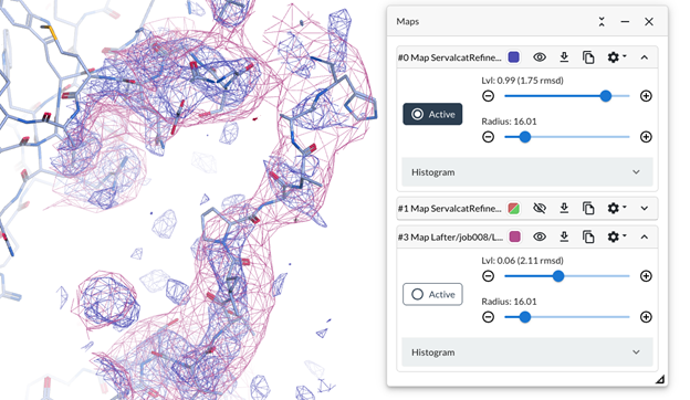
Create a selection between 726-737 and use the Refine button as before and see if the model improves the fit to the maps in this region. Remember that the “○ Active” button selects which map is used for the refinement.